
In the AI model race, is the newest GPU enough?
Can you get the performance you paid for just by deploying the latest GPU, NVIDIA’s Blackwell (B200)?
Unfortunately, no. An accelerator delivers its full performance only when the GPU compute software is rewritten to keep pace with the hardware. It’s the same reason FlashAttention (FA), the standard approach to accelerating self-attention, has restructured its kernels with every hardware generation—FA2 for Ampere, FA3 for Hopper, FA4 for Blackwell.
We deployed the latest B200s. Why didn’t the kernels deliver?
Training an AI model runs an enormous number of operations on the GPU, over and over. The program that actually carries out each of those operations is called a GPU kernel.
mamba-ssm, the open-source package that provides Mamba-2’s kernels, wasn’t taking advantage of the new hardware features the B200 introduced. Its heuristics were tuned around the A100—the newest GPU available when the kernel was written—and on the B200 those settings became a bottleneck in how resources were allocated.
Why optimize Mamba-2? Long context and hybrid architectures
As large-scale AI models have grown more capable, “how quickly and accurately a model handles long context” has become the core metric separating the competitive models from the rest.
But the Transformer architecture behind most of today’s models has a critical weakness. Because of how its core operation, self-attention, is structured, both computational complexity and key-value (KV) cache memory cost climb sharply as the input context grows longer.
What does that look like in practice?
Say you want to summarize a 500-page stack of dense legal documents in one pass, or feed in hours of high-resolution video and analyze it for anomalies. In long-context settings like these, a model built purely on conventional self-attention either runs out of memory (OOM) or slows to a crawl before it produces an answer.
To solve both problems at once—the “compute bottleneck” and the “memory blowup”—the global AI ecosystem is going through a significant technical shift.
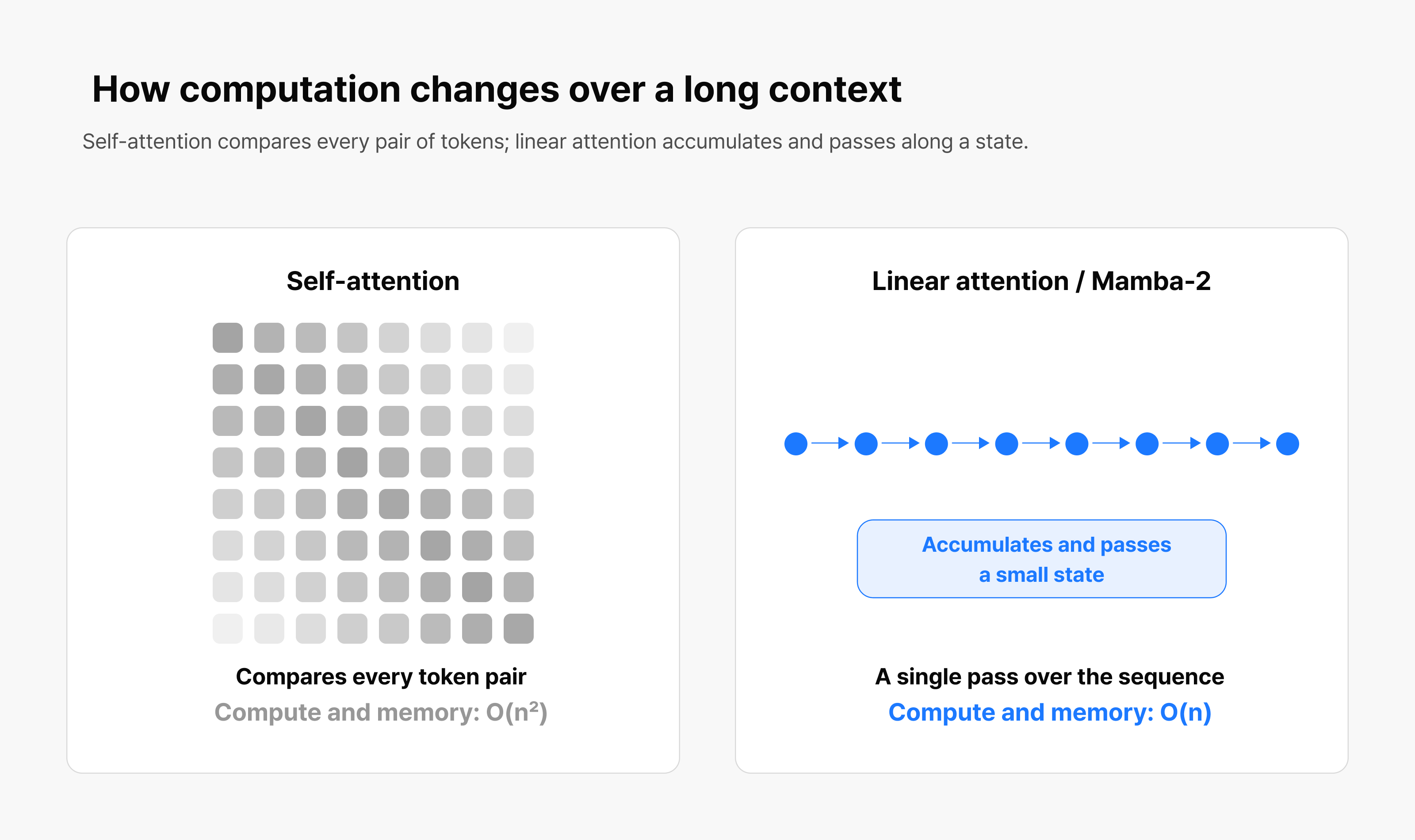
Figure 1. How self-attention and linear attention compute over a long context
Time and space complexity: self-attention vs. linear attention
| Self-attention | Linear attention (e.g., Mamba-2) | |
|---|---|---|
| Computational complexity | O(N²) (quadratic in sequence length) | O(N) (linear in sequence length) |
| KV cache memory | Blows up as the sequence grows (causes OOM) | Minimal, constant memory footprint |
State-of-the-art LLMs such as NVIDIA Nemotron, Alibaba Qwen, and Moonshot AI Kimi have begun adopting hybrid architectures in earnest: they keep the strengths of self-attention while blending in a fixed proportion of far more efficient linear attention layers (Mamba-2, GDN, KDA, and others). The result is a model that holds on to its language understanding and reasoning quality while cutting both computational complexity and KV cache memory pressure.
As architectures like Mamba-2 see wider use, how efficiently they run on the newest GPUs becomes just as important a question.
Building a Mamba-2 kernel for the B200: Why Helion?
To get real B200 performance out of the existing open-source kernels, we adopted Helion, a new DSL.
The reason comes down to one thing: Helion extends Triton’s autotuner so that it automatically searches for configuration values matched to the actual compute conditions—GPU architecture, input and output dimensions, data type. Three properties made the difference.
1. Preserved ecosystem compatibility
Helion is a domain-specific language (a language designed for one particular purpose) that layers an abstraction on top of Triton. That means we keep full compatibility with our existing PyTorch and Triton development logic while gaining far more freedom to redesign kernels.
2. A powerful built-in autotuner
Helion ships with an autotuning engine that helps apply the instructions and hardware features new to the B200—TMA, TMEM, warp specialization, and others—at the right points in the computation.
3. Automated heuristic optimization
Heuristic parameters that engineers used to hard-code by hand in Triton kernels become part of the autotuning search space, which lets us reach peak performance for a specific hardware target.
The optimization process: Find what’s slow → keep it accurate → rebuild it for the B200
Optimizing mamba-ssm’s kernels for the B200 wasn’t a series of quick one-off patches; it ran as a systematic three-stage process. We diagnosed the compute bottlenecks precisely, preserved numerical precision for model training, and, rather than leaving hardware features to the autotuner alone, reworked the logic and heuristics ourselves.
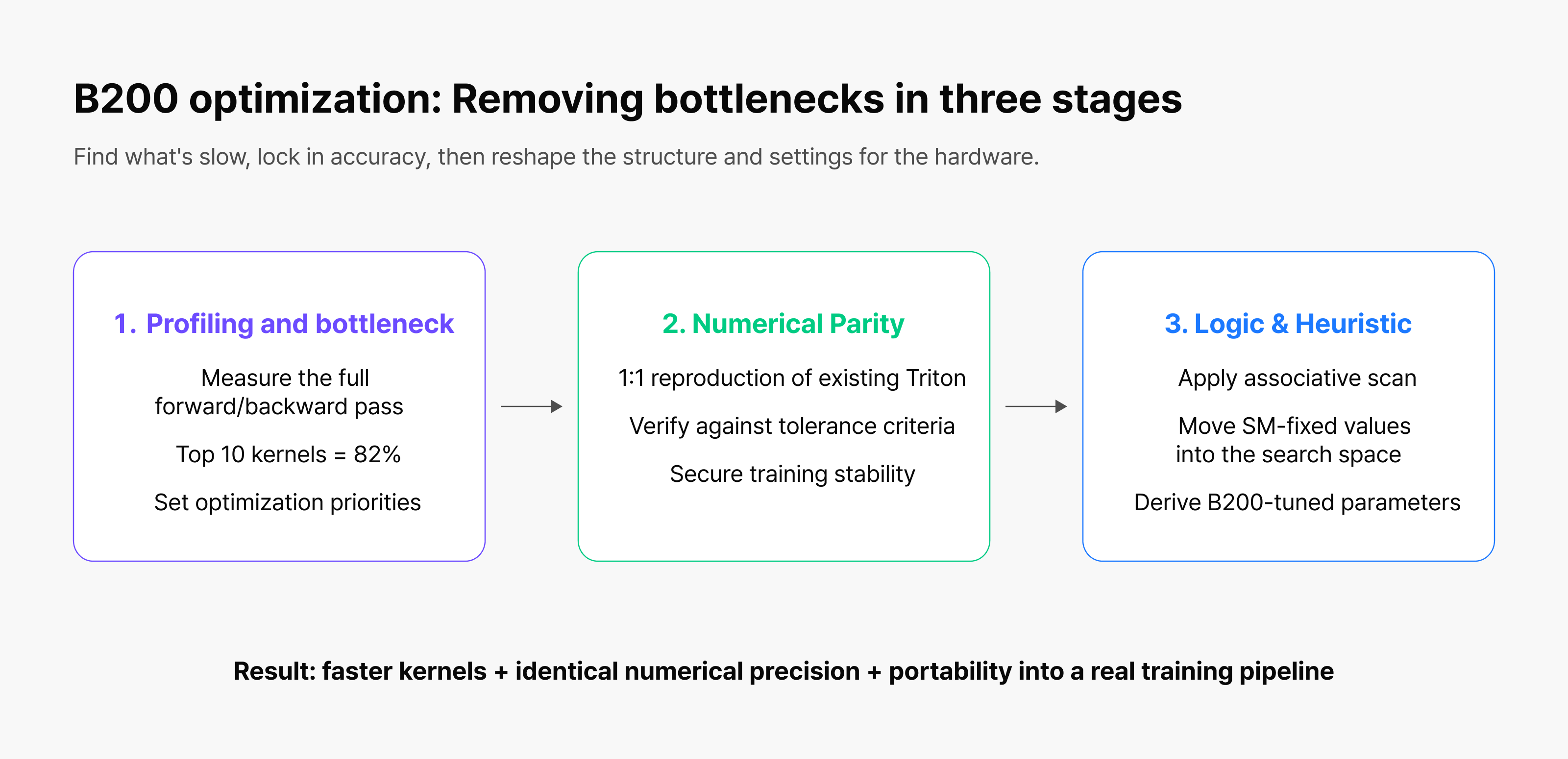
Figure 2. The three-stage optimization process: profiling and bottleneck analysis → numerical parity → logic and heuristic refinement
Stage 1. Profiling and bottleneck analysis
In the first stage we profiled, kernel by kernel, how much of the total compute each one accounted for across the full forward and backward passes of Mamba-2 training.
The top 10 kernels turned out to account for 82% of total compute time. Working from the profile, we picked out the worst bottlenecks first and prioritized them, so the least work would produce the largest latency reduction.
Share of compute time by kernel
The top 10 kernels account for 82% of total compute time.
| Kernel name | Phase + Step | % (Baseline) |
|---|---|---|
| _layer_norm_bwd | bwd_2 | 12.68 |
| _chunk_scan_fwd | fwd_5 | 12.32 |
| _chunk_scan_chunk_state_bwd_dx | bwd_10 | 10.81 |
| _chunk_scan_bwd_ddAcs_stable | bwd_16 | 9.43 |
| _chunk_state_fwd | fwd_2, bwd_5 | 9.25 |
| _chunk_scan_bwd_dC | bwd_12 | 6.09 |
| _chunk_state_bwd_db | bwd_11 | 6.04 |
| _state_passing_fwd | fwd_3, bwd_6 | 5.95 |
| _state_passing_bwd | bwd_9 | 5.54 |
| _chunk_scan_bwd_dstates | bwd_8 | 4.17 |
| Total | 82.28 |
Labels like bwd_2 and fwd_5 in the rest of this post refer to the Phase + Step column in the table above.
Stage 2. Numerical parity
However fast the kernels get, the optimization is worth little if precision errors creep in and training stops converging.
So before accelerating anything, we reproduced the exact arithmetic of the existing Triton implementation in Helion, one for one. We kept numerical error to a minimum and verified that stability held up in a large-scale training pipeline.
Stage 3. Logic and heuristic refinement
With numerical precision secured, we restructured the compute logic and parameters of several kernels to get the most out of the B200.
Adopting the associative scan primitive: A direct port of the sequential loops in _state_passing_fwd and _state_passing_bwd barely moved the needle, so we rebuilt them on Helion’s associative scan primitive, which maximized parallelism.
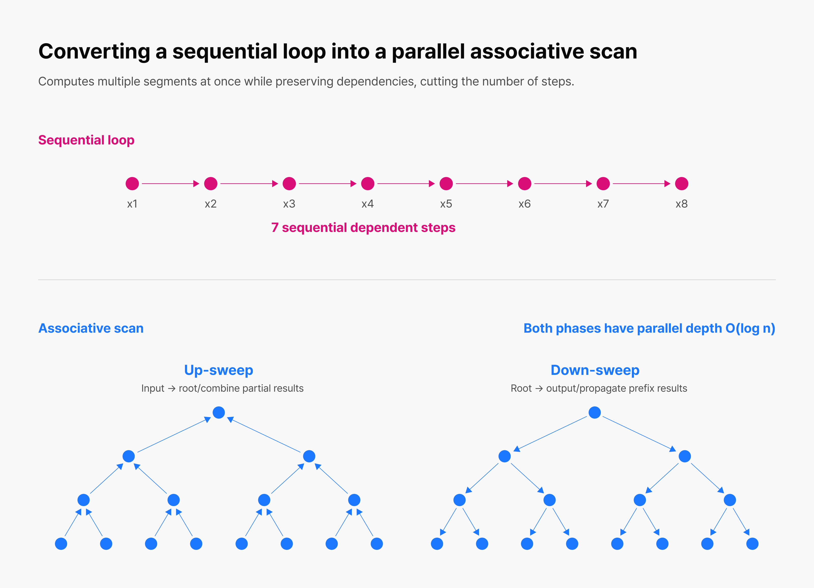
Figure 3. Execution steps in a sequential loop versus an associative scan
Reworking the SM-count heuristic: Heuristic parameters pinned to the GPU’s SM count can degrade performance on the B200. We added them to the autotuning search space so they adapt to the new environment. This was the change that mattered most.
From a fast kernel to a kernel we actually train with
That three-stage pipeline—profiling and bottleneck analysis, numerical parity, logic and heuristic refinement—substantially improved both the precision and the speed of individual kernels. But kernel optimization alone doesn’t finish the engineering. The next problem was how to fold these optimized kernels into a large-scale training pipeline without losing any of the gain, and in a form the team could keep building on.
Carrying the kernel-level gains through to real large-scale pre-training meant clearing two engineering barriers. The first was time overhead: every change to the model structure or batch configuration triggered one to two hours of autotuning. The second was portability and extensibility—making the kernels sit cleanly inside the existing training pipeline.
Cutting autotuning overhead with an automated config generator
Helion’s autotuning finds B200-optimized tiling and block hyperparameters on its own. But paying one to two hours of search time every time the training environment changes becomes a serious bottleneck when you’re running experiments constantly on a large cluster.
So we built an automated config generator that fully separates the autotuning search from the training run. It searches for the best tiling and block-size parameters for each training environment ahead of time and writes them to a file; pre-training then loads the stored config and starts immediately. Optimized kernel performance is available right away, with no one-to-two-hour wait.
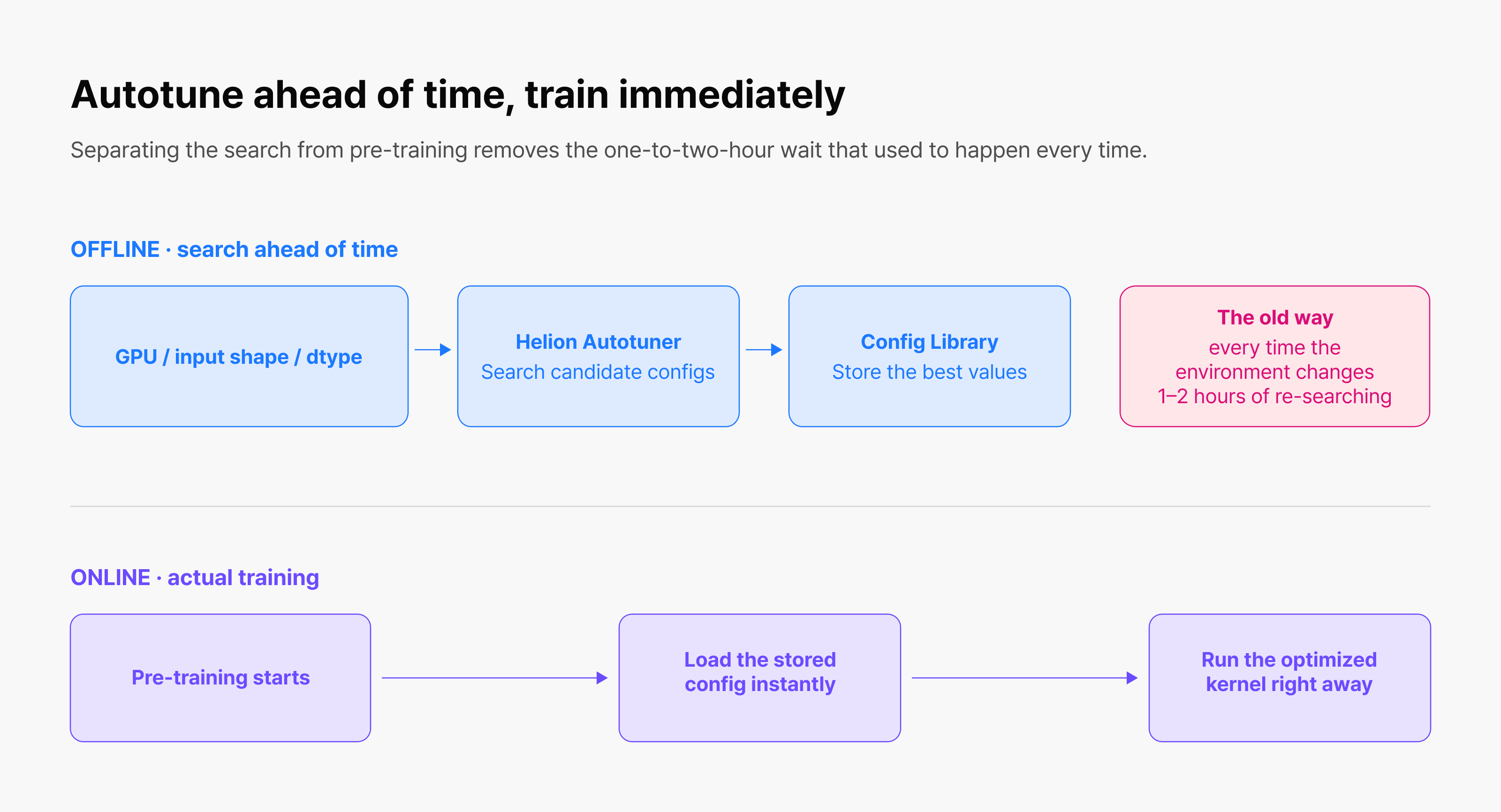
Figure 4. How configs found by offline autotuning are reused at training time
A one-for-one drop-in module and PyTorch/Triton portability
However good an optimized kernel is, it’s hard to put to work in day-to-day R&D if it doesn’t fit the existing training framework or demands sweeping code changes. So we designed our modules to drop straight into the open-source mamba-ssm package, one for one, giving us complete portability with PyTorch/Triton workflows.
That one-for-one structure buys us two practical advantages.
Fast numerical error tracing
Building on the precision we verified in the three-stage pipeline, we can quickly trace whether numerical error accumulates at scale, one layer at a time.
Reusable, extensible modules
The same kernel module can be reused without structural changes to the framework above it, which gives us a base we can extend easily—into context parallelism for long-context data, and into other distributed training paradigms.
So how much faster is it?
What did the three-stage optimization and the automation pipeline actually buy us on real hardware?
- The _layer_norm_bwd bottleneck kernel: up to 3.18x
- A single Mamba-2 layer (forward + backward): about 1.33x
- End-to-end Nemotron-3 Nano 30B pre-training: about 1.12x
For a single Mamba-2 layer (forward + backward), we hit a 1.33x speedup over the open-source mamba-ssm baseline.
Latency and speedup by kernel
In the table, Target is the top 10 kernels we optimized (82% of the total) and Total is the full layer. Every target kernel got faster, with speedups ranging from 1.20x to 3.18x.
| Phase + Step | % (Baseline) | Latency (Baseline, ms) | Latency (Helion, ms) | Speedup |
|---|---|---|---|---|
| bwd_2 | 12.68 | 0.28 | 0.09 | 3.18 |
| fwd_5 | 12.32 | 0.27 | 0.20 | 1.33 |
| bwd_10 | 10.81 | 0.24 | 0.19 | 1.22 |
| bwd_16 | 9.43 | 0.21 | 0.16 | 1.30 |
| fwd_2, bwd_5 | 9.25 | 0.20 | 0.15 | 1.33 |
| bwd_12 | 6.09 | 0.13 | 0.09 | 1.48 |
| bwd_11 | 6.04 | 0.13 | 0.10 | 1.31 |
| fwd_3, bwd_6 | 5.95 | 0.13 | 0.11 | 1.20 |
| bwd_9 | 5.54 | 0.12 | 0.09 | 1.32 |
| bwd_8 | 4.17 | 0.09 | 0.07 | 1.25 |
| Target the 10 kernels we optimized |
82.28 | 1.80 | 1.26 | 1.43 |
| Total the full layer |
100.00 | 2.18 | 1.64 | 1.33 |
Measurement conditions: a single B200, bf16, Nemotron-3 Nano 30B configuration, batch 2 / seqlen 8192. Median of 100 repeated runs after 10 warm-up iterations. mamba-ssm v2.3.1.
Tracking performance kernel by kernel, _layer_norm_bwd stood out with a 3.18x speedup.
The short version: no new algorithm was involved. A single configuration value, frozen at what made sense in the A100 era, was holding the B200 back—and this is what happened once we fixed it.
“The highway got wider, but we didn’t add any cars.”
Picture widening a highway from four lanes to sixteen. A single car still takes exactly as long to drive from Seoul to Busan. To see any benefit from the extra lanes, you have to put proportionally more cars on the road at the same time. Send through only as many as the four-lane road carried, and most of those sixteen lanes sit empty. That’s the situation the B200 was in.
_layer_norm_bwd is a textbook memory-bound operation—one whose performance is dictated by memory speed. Moving from the A100 to the B200, HBM bandwidth grew roughly 4 times, from 2 TB/s to 8 TB/s, but HBM latency didn’t fall by anything like the same factor.
That imbalance is the crux. If bandwidth quadruples while latency stays put, you have to issue proportionally more concurrent memory requests per SM to keep the pipe full. Fall short and the kernel is bound by latency rather than bandwidth—and in that state, no amount of extra hardware bandwidth helps.
How we fixed it
Triton’s existing heuristic sets its parameters aiming for “four warps per SM.” That’s a sensible target on the A100, but the B200 is a different machine. Apply the same heuristic to the B200’s 148 SMs and nrow_groups comes out at 74. The Helion autotuner, searching with the B200’s structure in view, settled on 2601—roughly 35 times larger. Concurrent memory requests jumped, latency was hidden, and performance improved 3.18 times.
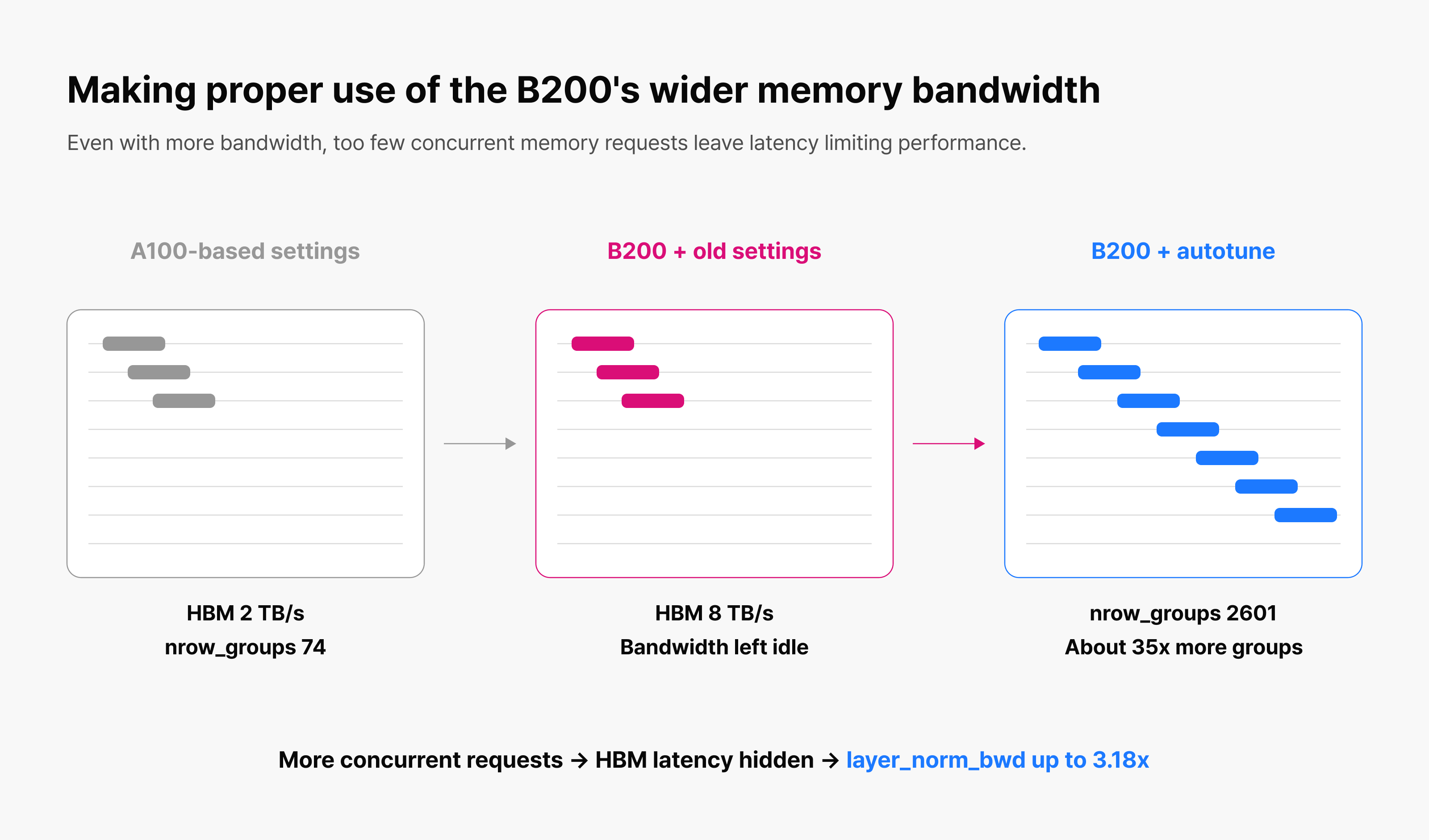
Figure 5. Why saturating the B200’s memory bandwidth requires more concurrent requests
What produced this gain wasn’t a new implementation technique but the parallelism parameter itself. Tuning that value by hand in the existing Triton kernel would likely get you a similar result.
Autotuning still mattered, though, because the parameter isn’t determined by SM count alone. The optimum also shifts with input dimensions, so a person would have to re-derive it every time the experimental setup changed. Automating that search is the practical benefit we got from adopting Helion.
What this case tells us
This work is less about introducing a new algorithm than about recovering performance the B200 had all along. For a kernel to get the full benefit of a hardware generation change, its parallelism parameters have to move with it. The size of the gain suggests the existing kernel wasn’t making full use of the B200’s memory bandwidth.
Faster kernels: Does the math still hold?
Speed is only worth having if the numbers stay right. To show that the gains came with no loss of precision, we ran precision checks based on the official mamba-ssm unit test suite.
Precision by phase and step
These are the differences between our outputs and those of the existing Triton implementation.
diff_mean: the mean absolute difference from the existing implementation, which tells us whether the new implementation is mathematically equivalent to the old one.
diff_max: the largest of those same differences, which tells us whether error spikes at any single point because of operation ordering or precision variation inside the kernel.
| Phase + Step | diff_mean | diff_max |
|---|---|---|
| bwd_2 | 2.24E-08 | 1.56E-02 |
| fwd_5 | 5.59E-09 | 1.56E-02 |
| bwd_10 | 4.78E-06 | 1.80E-02 |
| bwd_16 | 3.43E-07 | 2.77E-05 |
| fwd_2, bwd_5 | 2.84E-04 | 2.84E-04 |
| bwd_12 | 1.08E-08 | 2.86E-06 |
| bwd_11 | 3.51E-08 | 6.20E-06 |
| fwd_3, bwd_6 | 2.98E-08 | 6.10E-05 |
| bwd_9 | 1.40E-08 | 3.13E-02 |
| bwd_8 | 2.29E-07 | 6.01E-02 |
Verification criterion: |difference| ≤ atol + rtol × |reference| (atol = 1×10⁻², rtol = 1×10⁻²)
Result: across every forward and backward step, the mean absolute difference ranged from 5×10^-9 to 3×10^-4.
End-to-end validation: Nemotron-3 Nano 30B training
Beyond the single-layer benchmark, we dropped the optimized kernels one for one into a live pre-training pipeline—the Nemotron-3 Nano 30B (A3B) training environment—and validated them end to end.
Shorter iteration time
At the whole-model level, each training step ran 1.12x faster, which translates into real savings in large-cluster time and cost.
Loss convergence preserved
The loss curve tracks that of the baseline kernel. Over long training runs of hundreds of thousands of steps, the kernels ran stably with no NaNs and no loss spikes.
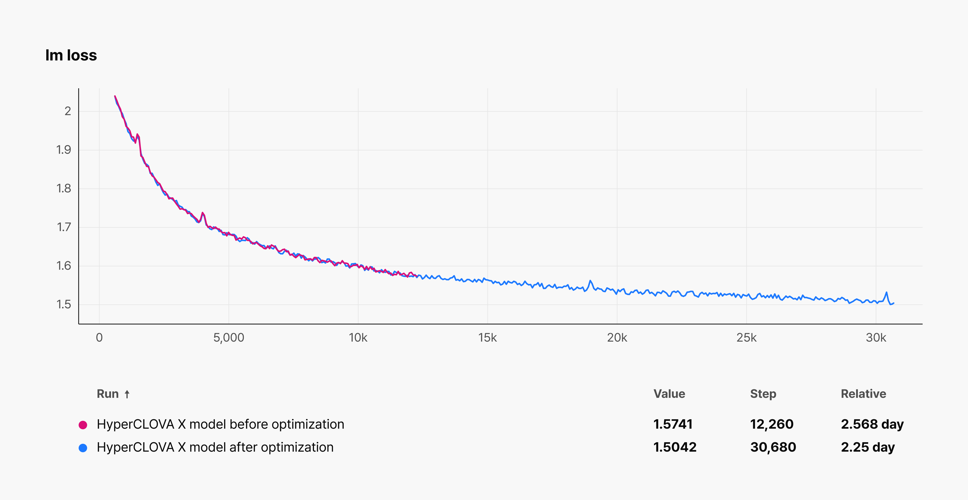
Figure 6. Training loss for the baseline and Helion-optimized kernels over training steps
Validation setup: 32 nodes, global batch 3072, sequence length 8192, tensor parallel 2, expert parallel 8. Nemotron-3 Nano 30B (A3B), bf16.
Closing thoughts: Securing GPUs isn’t the same as unlocking them
Deploying a state-of-the-art accelerator like the B200 isn’t enough on its own to lead in the era of large-scale AI. Leading also takes in-house expertise in the core kernel software that actually draws out the hardware’s latent performance.
With Helion-based Mamba-2 kernel optimization tailored to the B200, NAVER Cloud has demonstrated concrete numbers: 1.33x on a single layer and 1.12x on end-to-end training.
We’ll extend the gains validated on Nemotron-3 Nano 30B to larger models in our lineup. With even more extreme sequence lengths in view, we’re researching how to connect these Helion Mamba-2 kernels to context parallelism and multi-node GPU cluster environments, so that efficiency scales horizontally across a whole cluster rather than stopping at a single node.
NAVER Cloud will keep bringing together forward-looking research on AI model architecture and next-generation accelerator software optimization, building a compute-efficient, sovereign AI infrastructure ecosystem.