
In our previous post, “Inside LLM serving (1),” we explored how LLMs work and why tokens and GPUs are fundamental to their operation. In this second installment, we’ll trace the complete path of a user’s prompt as it flows through the server, examine how responses are generated, and understand why memory (specifically KV cache) becomes a critical factor determining serving performance. We’ll analyze this through two key performance indicators—latency and throughput—to tackle LLM serving’s central challenge: processing more requests faster.
Latency and throughput: Core performance metrics for LLM serving
Deploying an LLM service successfully requires more than just getting it off the ground—you must balance user experience with system efficiency. This balance hinges on two critical performance metrics: latency and throughput.
Latency
Latency measures the time from when a user sends a request to when they receive a response—essentially, their perceived responsiveness. For LLMs, latency breaks down into two parts:
- Time to first token (TTFT): The delay before users see the first token appear on their screen. This is largely determined by initial computation in understanding the prompt.
- Time per output token (TPOT): The average time required to generate each subsequent token after the first. Since total response time approximates TTFT + (TPOT × number of output tokens), longer responses naturally take more time to complete.
Throughput
Throughput measures how many requests your system can process within a given timeframe, typically expressed as tokens per second in LLM serving. Higher throughput means your system can efficiently handle more concurrent users.
The latency-throughput trade-off
These metrics often pull in opposite directions. Dedicating system resources to minimize one user’s latency can force other users to wait longer, reducing overall throughput. Conversely, maximizing throughput through techniques like request batching (processing multiple requests together) increases individual wait times, thereby increasing latency. Successful LLM service design requires finding the right balance for your workload characteristics and requirements.
KV cache and memory usage: Enabling fast inference
During the decode phase, recalculating past data from scratch for every new token would be computationally wasteful. To solve this, LLMs employ a mechanism called KV cache—essentially a “notepad” that stores intermediate attention results (keys and values) in GPU memory. When generating the next token, the model reuses these cached values instead of recomputing everything, dramatically accelerating the process.
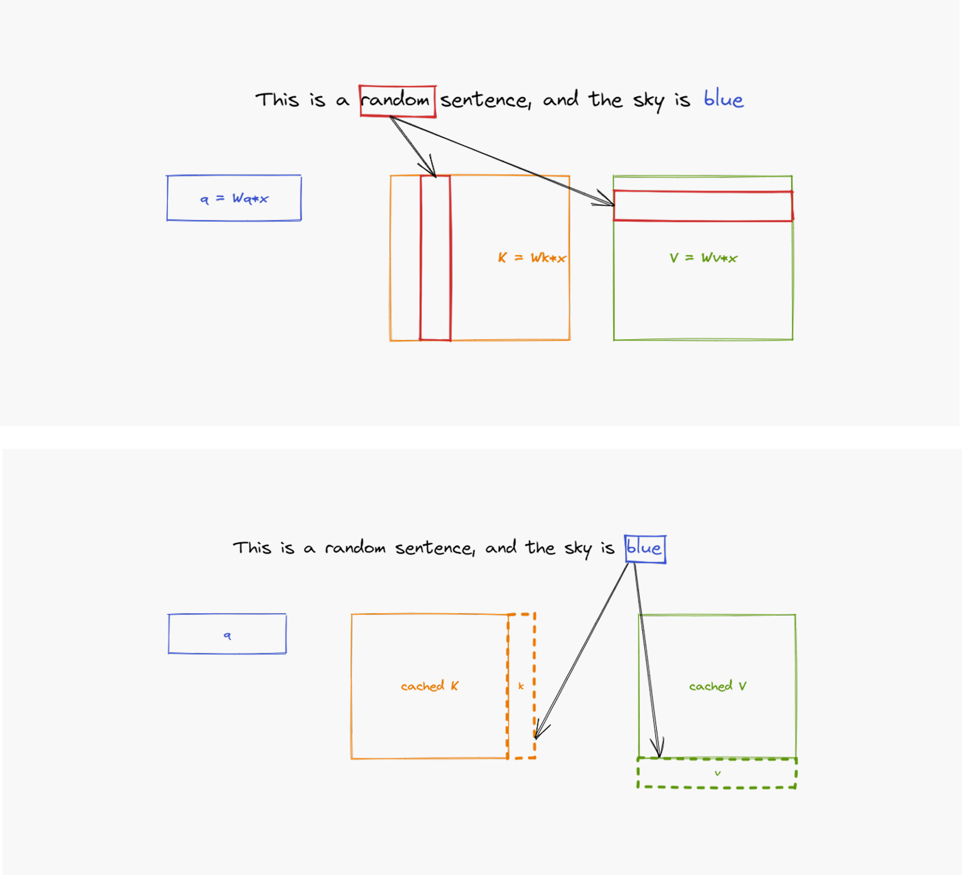
[Figure 1]: Each layer stores token calculations in cache to avoid redundant computation when generating subsequent tokens (source: What is the KV cache?)
Why larger models slow down
Memory bandwidth becomes the bottleneck as models scale. Larger models require reading more weights from high-bandwidth memory (HBM), while additional layers and larger hidden dimensions expand the KV cache size. As the volume of data that must be read and written increases with each token generation, decode speed inevitably drops.
The cost of caching
KV cache consumes substantial GPU memory, calculated approximately as:
KV cache memory (bytes) ≈ [batch size] × [sequence length] × [layers] × [hidden size] × 2 (K, V) × [data type size]
Where:
- Batch size: Number of concurrent requests
- Sequence length: Input tokens + generated tokens
- Number of layers: Model depth
- Hidden size: Internal vector dimensions
- Data type size: 2 bytes for BF16
If you know the memory size of the model weights, you can estimate the number of tokens that can be stored in a fixed GPU memory (Batch size × Sequence length). Total GPU memory usage becomes: Model weights + KV cache memory. This sum constrains how many requests you can process simultaneously and their maximum length, directly impacting latency.
The batch size vs. sequence length trade-off
Within fixed GPU memory, you face an unavoidable choice:
- Increase batch size to handle more concurrent requests, but reduce the sequence length available to each.
- Support lengthy sequences (like document summarization) by reducing batch size, limiting concurrent users.
Think of GPU memory as a fixed-size container. Short sequences are like small items—you can pack many efficiently. Long sequences consume most of the available space, like large objects in a container, limiting how many you can process simultaneously.
Processing together: The benefits and constraints of batching
To maximize GPU parallel processing capabilities, LLM serving systems use batching—grouping multiple user requests for simultaneous processing. Generally, larger batch sizes improve GPU utilization and increase overall throughput.
However, batch size growth faces two fundamental constraints that create practical limits.
Constraint 1: Finite GPU memory
GPU memory creates the first bottleneck. As batch size increases, the memory footprint grows proportionally—while model weights remain constant, KV cache size scales directly with the number of concurrent requests. This expanding cache eventually exhausts available GPU memory, establishing a hard limit on how large batches can grow.
Constraint 2: Latency service-level objectives
The second constraint comes from latency requirements, or service-level objectives (SLOs). Processing larger batches increases the KV cache that must be read and written during each generation step. Even though you’re handling more tokens per batch, the time required to process that batch grows correspondingly.
We’ll examine this latency-throughput trade-off in detail in the next section.
Goodput determines LLM performance
We’ve established that throughput and latency exist in tension with each other. But how do we measure real-world performance when both metrics matter? Enter goodput—a metric that counts only responses meeting latency requirements (SLO), showing how many usable responses are delivered within a given timeframe. Goodput captures both speed and volume in one practical measurement.
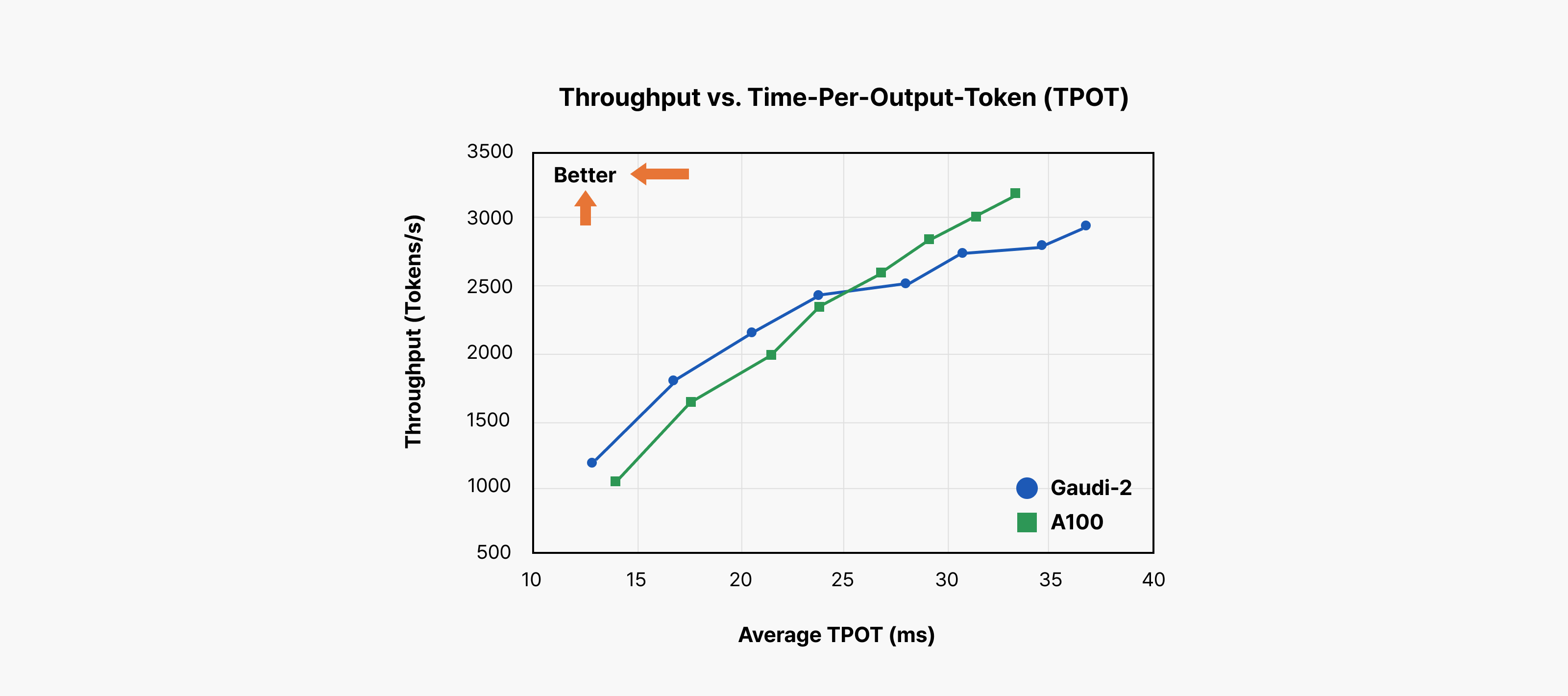
[Figure 2]: Throughput vs. time-per-output token (source: Intel Gaudi Introduction)
This chart reveals how well an LLM serving system actually performs:
- X-axis (Time per output token): Average time to generate a single token, also called inter-token latency (ITL). Points further left indicate faster token generation.
- Y-axis (Output token throughput): Total tokens the system generates per second. Higher positions indicate more concurrent request handling.
Ideally, systems should occupy the top-left region: fast response times (low latency) while processing many users simultaneously (high throughput).
Translating the ideal into goodput
Goodput quantifies this ideal. Unlike raw throughput, goodput measures throughput achieved while meeting latency SLOs—throughput that doesn’t compromise user experience.
Consider an SLO requiring “average token generation under 20ms” for optimal user experience. Draw a vertical line at the 20ms point on the x-axis. Where each hardware/configuration performance curve intersects this line represents that system’s achievable goodput within the SLO. You could push throughput higher, but beyond 20ms, users perceive slowness. Throughput beyond this point becomes “badput“—it degrades user experience rather than improving service quality.
Sequence length impacts goodput
Goodput varies dramatically based not only on model size but also sequence length. Long conversations, document summarization, or accumulated multi-turn interactions create extended sequences. This increases the KV cache that must be accessed during each token generation. Larger KV cache increases inter-token latency, shifting the entire performance curve rightward. Consequently, the same 20ms SLO line intersects at lower throughput values—reducing goodput.
Comparing performance fairly
When evaluating LLM service performance, context matters:
- Which latency SLO was used for measurement?
- What sequence length was tested?
Identical models can show vastly different performance under different conditions, directly affecting real user experience.
Goodput optimization: Understanding computation and memory bottlenecks
To build effective LLM serving systems, you must first accurately diagnose “Where is this system slowing down?” LLM inference performance degrades for two fundamental reasons:
- Compute-bound scenarios
Performance is limited by the computational capacity of arithmetic units like GPU cores. The system has abundant computation to process, keeping the GPU fully utilized, but tasks take longer because there’s simply too much work for the available processing power. - Memory-bound scenarios
Performance is constrained by data access rather than computation. The GPU sits idle, waiting for the data needed for operations to arrive from memory. Here, memory bandwidth—particularly HBM bandwidth—determines overall performance, not computational throughput.
LLM inference exhibits these characteristics distinctly across its two phases:
- Prefill phase: Compute-bound
When processing user input, the LLM handles the entire prompt through large-scale parallel matrix operations. Performance depends on how much computation the GPU can execute simultaneously. - Decode phase: Memory-bound
Token generation involves lighter computation since tokens are produced sequentially, but requires continuously reading large model weights and accumulated KV cache from memory. The bottleneck shifts from computation to data access speed—memory bandwidth and cache management become more critical than computational performance.
Effective goodput improvement requires first identifying your current bottleneck. Is your workload compute-bound or memory-bound? This diagnosis determines your optimization path: reducing computational overhead, compressing or sharing KV cache, or adjusting batching strategies.
Bottleneck solving strategies
Now that we’ve identified the bottlenecks, let’s examine targeted approaches for addressing each constraint.
High-bandwidth memory: Addressing memory-bound constraints
The memory-bound nature of the decode phase explains why high-bandwidth memory (HBM) is critical for LLM GPUs.
During single token generation, the GPU must read tens to hundreds of gigabytes of model weights and KV cache from HBM. HBM’s data transfer speed directly determines inter-token latency (ITL)—no matter how fast your computation, insufficient memory bandwidth will constrain overall performance.
Crucially, batch size affects model weights and KV cache differently. Model weights represent a fixed data volume regardless of batch size, so batching can amortize this cost across multiple requests. However, KV cache grows proportionally with batch size, increasing rather than sharing the memory I/O burden and often becoming the primary system constraint.
Systolic arrays: Solving compute-bound constraints
To address compute-bound bottlenecks in the prefill phase, modern AI accelerators include dedicated matrix operation hardware. Systolic arrays exemplify this approach—they enable data to flow in regular patterns while computation proceeds continuously, facilitating efficient large-scale matrix operations.
NVIDIA’s Tensor Cores represent this systolic array design, handling significantly more matrix operations than general GPU cores and dramatically accelerating prefill phase processing.
Parallel processing: Scaling beyond single GPU limits
When single-GPU performance falls short of desired goodput, multi-GPU parallel processing becomes essential. Multiple GPUs improve not only computation but also memory bandwidth substantially.
Consider distributing an LLM across 4 GPUs: each handles one-quarter of the model, and during inference, all four read data simultaneously from their respective HBMs. Theoretically, this quadruples memory access speed—particularly beneficial for reducing latency in memory-bound scenarios like the decode phase.
However, parallel processing introduces new constraints. Multi-GPU coordination requires inter-GPU communication, and communication bandwidth (e.g., NVLink) can create fresh bottlenecks. Additionally, data synchronization demands computational overhead, preventing linear performance scaling with additional GPUs.
Algorithm enhancement: Software-level optimizations
Beyond hardware and system techniques, algorithmic improvements significantly accelerate LLM inference. Speculative decoding illustrates this approach: a small, fast model generates several candidate tokens, then a larger, more accurate model verifies and refines these predictions in parallel. The small model creates a “quick draft” while the larger model “reviews and confirms” it simultaneously, reducing overall response time.
Other active research areas include conditional computation (selectively executing required operations), cache optimization through intermediate computation reuse, and adaptive decoding strategies. These techniques share a common goal: achieving higher goodput with identical resources by optimizing the latency-throughput trade-off.
Algorithm enhancements prove most effective when combined with hardware and system optimizations.
For deeper insights, see our earlier post on speculative decoding.
Final goal: Tokens per dollar
We’ve explored numerous technologies that enhance speed and processing capacity. In practice, however, cost matters just as much as performance when operating LLMs. No matter how exceptional the performance, prohibitively high operational costs eliminate practical value.
Therefore, the ultimate objective for LLM serving should be maximizing tokens per dollar—an efficiency metric that captures both system processing performance (tokens per second) and total operational costs (hardware, electricity, and infrastructure expenses).
The core challenge isn’t simply selecting the fastest GPU, but finding the optimal hardware and software combination that achieves your defined goodput targets at minimum cost.
References
For deeper insights into LLM serving economics and optimization:
TensorEconomics. “LLM Inference Economics from First Principles.” https://www.tensoreconomics.com/p/llm-inference-economics-from-first
SemiAnalysis. “InferenceMAX™: Open Source Inference Benchmarking.” https://newsletter.semianalysis.com/p/inferencemax-open-source-inference